The assumption that a VNM expected utility function is linear in probabilities, though not in payoffs, allows us to create an indifference-curve representation.

To create a simple two-dimensional representation, let's assume we have only 3 possible outcomes, x₁, x₂, and x₃, such that x₁ x₂ x₃. Assume they occur with probabilities p₁, p₂, and p₃ respectively, where p_i = 1.

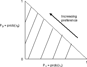
Now, since p₂ = 1 - p₁ - p₃, we can represent these lotteries by points in a unit triangle in the (p₁, p₃) plane, known as the Machina triangle.

Upward movements in the triangle increase p₃ at the expense of p₂, shifting probability from x₂ to x₃. Leftward movements reduce p₁ to the benefit of p₂, shifting probability from from x₁ to x₂. As a result, both of these, and more generally, all northwest movements, lead to stochastically dominating lotteries that will be preferred.

Since the indifference curves are given by solutions to the linear equation:

u* = U(x₁)p₁ + U(x₂)(1 - p₁ - p₃) + U(x₃)p₃ = constant,

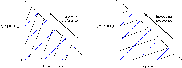
they consist of parallel straight lines of slope [U(x₂) - U(x₁)]/[U(x₃) - U(x₂)]. As a result, we can use this type of diagram to illustrate attitudes to risk, as under:

The blue lines in both panels are iso-expected value lines, while the black lines are indifference curves. The iso-expected value lines are, of course, the solutions to:

x* = x₁p₁ + x₂(1 - p₁ - p₃) + x₃p₃ = constant

Northeast movements along the blue lines do not change the expected value of the prospect, but they increase the probabilities of of the tail outcomes x₁ and x₃. They are mean-preserving spreads, or pure increases in risk. The left-hand panel contains indifference curves much steeper than the the iso-expected value lines, so they are indifference curves formed by the concave utility function of a risk-averse individual. In the right-hand panel, the indifference curves are much flatter than the iso-expected value lines. This implies that they are representations of the risk-loving preferences of an individual with a convex utility function. Similarly, a risk-neutral individual would have indifference curves that coincide with the iso-expected value lines.

Linearity in probabilities implies and is implied by the substitution or independence axiom. The famed Allais Paradox is the best example of systematic violations of this axiom.

Recall that subjects choose from the following:
Gamble A: A 100% chance of receiving $1 million
Gamble B: A 10% chance of receiving $5 million, an 89% chance of receiving $1 million, and a 1% chance of receiving nothing.

They then choose between:
Gamble C: An 11% chance of receiving $1 million, and an 89% chance of receiving nothing
Gamble D: A 10% chance of receiving $5 million, and a 90% chance of receiving nothing.

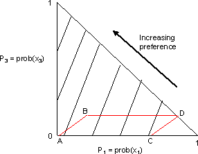
Most subjects choose A in the first round and D in the second. However, preferring A in the first round to B implies steep indifference curves, so the independence axiom would require that one choose C in the second round, not D. If one chooses D in the second round, the implication is that one's indifference curves are flat, and B should be chosen in the first round. This is illustrated below:

We can see that the 4 gambles form a parallelogram in the Machina triangle, where outcome x₁ is a payoff of 0, outcome x₂ is a payoff of $1 million, and outcome x₃ is a payoff of $5 million.

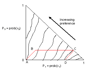
We can see that a person's indifference curves appear to be steep in the first case, and flat in the second - they fan out, as under, and are not parallel.

Originally, the Allais Paradox was considered an isolated example, but further experimental testing has shown it to be part of a general empirical pattern, called the common consequence effect. The effect involves any pairs of probability mixtures of the form:

A: ad_x + (1-a)P**, versus B: aP + (1-a)P**;

and

C: ad_x + (1-a)P*, versus D: aP + (1-a)P*.

Here, d_x denotes the lottery yielding x with certainty. P is a lottery involving outcomes both greater and less than x. P** stochastically dominates P*, i.e. the more preferred outcome has a higher probability, and the less preferred outcome has a lower probability, in P** than in P*. When the distributions are over a common outcome set, say x₁, x₂, and x₃, the prospects will form a parallelogram in the probability triangle, as above. Any choice of A and D will once again imply indifference curves which fan out.

1. Machina, Mark J. (1987), "Choice Under Uncertainty: Problems Solved and Unsolved," Journal of Economic Perspectives, Vol. 1, No. 1